2.4 Mutable Data
We have seen how abstraction is vital in helping us to cope with the complexity of large systems. Effective program synthesis also requires organizational principles that can guide us in formulating the overall design of a program. In particular, we need strategies to help us structure large systems so that they will be modular, that is, so that they can be divided "naturally" into coherent parts that can be separately developed and maintained.
One powerful technique for creating modular programs is to introduce new kinds of data that may change state over time. In this way, a single data object can represent something that evolves independently of the rest of the program. The behavior of a changing object may be influenced by its history, just like an entity in the world. Adding state to data is an essential ingredient of our final destination in this chapter: object-oriented programming.
The native data types we have introduced so far — numbers, Booleans, tuples, ranges, and strings — are all types of immutable objects. While names may change bindings to different values in the environment during the course of execution, the values themselves do not change. Mutable objects (also called mutable values) can change throughout the execution of a program.
2.4.1 Lists
The list is Python's most useful and flexible sequence type. A list is similar to a tuple, but it is mutable: Method calls and assignment statements can change the contents of a list.
We can introduce many list modification operations through an example that illustrates the history of playing cards (drastically simplified). Comments in the examples describe the effect of each method invocation.
Playing cards were invented in China, perhaps around the 9th century. An early deck had three suits, which corresponded to denominations of money.
>>> chinese_suits = ['coin', 'string', 'myriad']  # A list literal
>>> suits = chinese_suits                         # Two names refer to the same list
As cards migrated to Europe (perhaps through Egypt), only the suit of coins remained in Spanish decks (oro).
>>> suits.pop()             # Remove and return the final element
'myriad'
>>> suits.remove('string')  # Remove the first element that equals the argument
Three more suits were added (they evolved in name and design over time),
>>> suits.append('cup')              # Add an element to the end
>>> suits.extend(['sword', 'club'])  # Add all elements of a list to the end
and Italians called swords spades.
>>> suits[2] = 'spade' # Replace an element
giving the suits of a traditional Italian deck of cards.
>>> suits
['coin', 'cup', 'spade', 'club']
The French variant that we use today in the U.S. changes the first two:
>>> suits[0:2] = ['heart', 'diamond']  # Replace a slice
>>> suits
['heart', 'diamond', 'spade', 'club']
Methods also exist for inserting, sorting, and reversing lists. All of these mutation operations change the value of the list; they do not create new list objects.
Sharing and Identity. Because we have been changing a single list rather than creating new lists, the object bound to the name chinese_suits has also changed, because it is the same list object that was bound to suits!
>>> chinese_suits  # This name co-refers with "suits" to the same list
['heart', 'diamond', 'spade', 'club']
This behavior is new. Previously, if a name did not appear in a statement, then its value would not be affected by that statement. With mutable data, methods called on one name can affect another name at the same time.
The environment diagram for this example shows how the value bound to chinese is changed by statements involving only suits. Step through each line of the following example to observe these changes.
Lists can be copied using the list constructor function. Changes to one list do not affect another, unless they share structure.
>>> nest = list(suits)  # Bind "nest" to a second list with the same elements
>>> nest[0] = suits     # Create a nested list
According to this environment, changing the list referenced by suits will affect the nested list that is the first element of nest, but not the other elements.
>>> suits.insert(2, 'Joker')  # Insert an element at index 2, shifting the rest
>>> nest
[['heart', 'diamond', 'Joker', 'spade', 'club'], 'diamond', 'spade', 'club']
And likewise, undoing this change in the first element of nest will change suit as well.
>>> nest[0].pop(2)
'Joker'
>>> suits
['heart', 'diamond', 'spade', 'club']
Stepping through this example line by line will show the representation of a nested list.
Because two lists may have the same contents but in fact be different lists, we require a means to test whether two objects are the same. Python includes two comparison operators, called is and is not, that test whether two expressions in fact evaluate to the identical object. Two objects are identical if they are equal in their current value, and any change to one will always be reflected in the other. Identity is a stronger condition than equality.
>>> suits is nest[0]
True
>>> suits is ['heart', 'diamond', 'spade', 'club']
False
>>> suits == ['heart', 'diamond', 'spade', 'club']
True
The final two comparisons illustrate the difference between is and ==. The former checks for identity, while the latter checks for the equality of contents.
List comprehensions. A list comprehension uses an extended syntax for creating lists, analogous to the syntax of generator expressions.
For example, the unicodedata module tracks the official names of every character in the Unicode alphabet. We can look up the characters corresponding to names, including those for card suits.
>>> from unicodedata import lookup
>>> [lookup('WHITE ' + s.upper() + ' SUIT') for s in suits]
['♡', '♢', '♤', '♧']
List comprehensions reinforce the general approach of sequence processing, as list is a sequence data type.
2.4.2 Dictionaries
Dictionaries are Python's built-in data type for storing and manipulating correspondence relationships. A dictionary contains key-value pairs, where both the keys and values are objects. The purpose of a dictionary is to provide an abstraction for storing and retrieving values that are indexed not by consecutive integers, but by descriptive keys.
Strings commonly serve as keys, because strings are our conventional representation for names of things. This dictionary literal gives the values of various Roman numerals.
>>> numerals = {'I': 1.0, 'V': 5, 'X': 10}
Looking up values by their keys uses the element selection operator that we previously applied to sequences.
>>> numerals['X']
10
A dictionary can have at most one value for each key. Adding new key-value pairs and changing the existing value for a key can both be achieved with assignment statements.
>>> numerals['I'] = 1
>>> numerals['L'] = 50
>>> numerals
{'I': 1, 'X': 10, 'L': 50, 'V': 5}
Notice that 'L' was not added to the end of the output above. Dictionaries are unordered collections of key-value pairs. When we print a dictionary, the keys and values are rendered in some order, but as users of the language we cannot predict what that order will be.
Dictionaries can appear in environment diagrams as well.
The dictionary abstraction also supports various methods of iterating of the contents of the dictionary as a whole. The methods keys, values, and items all return iterable values.
>>> sum(numerals.values())
66
A list of key-value pairs can be converted into a dictionary by calling the dict constructor function.
>>> dict([(3, 9), (4, 16), (5, 25)])
{3: 9, 4: 16, 5: 25}
Dictionaries do have some restrictions:
- A key of a dictionary cannot be an object of a mutable built-in type.
- There can be at most one value for a given key.
This first restriction is tied to the underlying implementation of dictionaries in Python. The details of this implementation are not a topic of this text. Intuitively, consider that the key tells Python where to find that key-value pair in memory; if the key changes, the location of the pair may be lost.
The second restriction is a consequence of the dictionary abstraction, which is designed to store and retrieve values for keys. We can only retrieve the value for a key if at most one such value exists in the dictionary.
A useful method implemented by dictionaries is get, which returns either the value for a key, if the key is present, or a default value. The arguments to get are the key and the default value.
>>> numerals.get('A', 0)
0
>>> numerals.get('V', 0)
5
Dictionaries also have a comprehension syntax analogous to those of lists and generator expressions. Evaluating a dictionary comprehension yields a new dictionary object.
>>> {x: x*x for x in range(3,6)}
{3: 9, 4: 16, 5: 25}
2.4.3 Local State
Lists and dictionaries have local state: they are changing values that have some particular contents at any point in the execution of a program. The word state implies an evolving process in which that state may change.
Functions can also have local state. For instance, let us define a function that models the process of withdrawing money from a bank account. We will create a function called withdraw, which takes as its argument an amount to be withdrawn. If there is enough money in the account to accommodate the withdrawal, then withdraw will return the balance remaining after the withdrawal. Otherwise, withdraw will return the message 'Insufficient funds'. For example, if we begin with $100 in the account, we would like to obtain the following sequence of return values by calling withdraw:
>>> withdraw(25)
75
>>> withdraw(25)
50
>>> withdraw(60)
'Insufficient funds'
>>> withdraw(15)
35
Above, the expression withdraw(25), evaluated twice, yields different values. Thus, this user-defined function is non-pure. Calling the function not only returns a value, but also has the side effect of changing the function in some way, so that the next call with the same argument will return a different result. This side effect is a result of withdraw making a change to a name-value binding outside of its local environment frame.
For withdraw to make sense, it must be created with an initial account balance. The function make_withdraw is a higher-order function that takes a starting balance as an argument. The function withdraw is its return value.
>>> withdraw = make_withdraw(100)
An implementation of make_withdraw requires a new kind of statement: a nonlocal statement. When we call make_withdraw, we bind the name balance to the initial amount. We then define and return a local function, withdraw, which updates and returns the value of balance when called.
>>> def make_withdraw(balance):
        """Return a withdraw function that draws down balance with each call."""
        def withdraw(amount):
            nonlocal balance                 # Declare the name "balance" nonlocal
            if amount > balance:
                return 'Insufficient funds'
            balance = balance - amount       # Re-bind the existing balance name
            return balance
        return withdraw
The novel part of this implementation is the nonlocal statement, which mandates that whenever we change the binding of the name balance, the binding is changed in the first frame in which balance is already bound. Recall that without the nonlocal statement, an assignment statement would always bind a name in the first frame of the environment. The nonlocal statement indicates that the name appears somewhere in the environment other than the first (local) frame or the last (global) frame.
The following environment diagrams illustrate the effects of multiple calls to a function created by make_withdraw.
The first def statement has the usual effect: it creates a new user-defined function and binds the name make_withdraw to that function in the global frame. The subsequent call to make_withdraw creates and returns a locally defined function withdraw. The name balance is bound in the parent frame of this function. Crucially, there will only be this single binding for the name balance throughout the rest of this example.
Next, we evaluate an expression that calls this function, bound to the name wd, on an amount 5. The body of withdraw is executed in a new environment that extends the environment in which withdraw was defined. Tracing the effect of evaluating withdraw illustrates the effect of a nonlocal statement in Python: a name outside of the first local frame can be changed by an assignment statement.
The nonlocal statement changes all of the remaining assignment statements in the definition of withdraw. After executing nonlocal balance, any assignment statement with balance on the left-hand side of = will not bind balance in the first frame of the current environment. Instead, it will find the first frame in which balance was already defined and re-bind the name in that frame. If balance has not previously been bound to a value, then the nonlocal statement will give an error.
By virtue of changing the binding for balance, we have changed the withdraw function as well. The next time it is called, the name balance will evaluate to 15 instead of 20. Hence, when we call withdraw a second time, we see that its return value is 12 and not 17. The change to balance from the first call affects the result of the second call.
The second call to withdraw does create a second local frame, as usual. However, both withdraw frames have the same parent. That is, they both extend the environment for make_withdraw, which contains the binding for balance. Hence, they share that particular name binding. Calling withdraw has the side effect of altering the environment that will be extended by future calls to withdraw. The nonlocal statement allows withdraw to change a name binding in the make_withdraw frame.
Ever since we first encountered nested def statements, we have observed that a locally defined function can look up names outside of its local frames. No nonlocal statement is required to access a non-local name. By contrast, only after a nonlocal statement can a function change the binding of names in these frames.
Practical Guidance. By introducing nonlocal statements, we have created a dual role for assignment statements. Either they change local bindings, or they change nonlocal bindings. In fact, assignment statements already had a dual role: they either created new bindings or re-bound existing names. Assignment can also change the contents of lists and dictionaries. The many roles of Python assignment can obscure the effects of executing an assignment statement. It is up to you as a programmer to document your code clearly so that the effects of assignment can be understood by others.
Python Particulars. This pattern of non-local assignment is a general feature of programming languages with higher-order functions and lexical scope. Most other languages do not require a nonlocal statement at all. Instead, non-local assignment is often the default behavior of assignment statements.
Python also has an unusual restriction regarding the lookup of names: within the body of a function, all instances of a name must refer to the same frame. As a result, Python cannot look up the value of a name in a non-local frame, then bind that same name in the local frame, because the same name would be accessed in two different frames in the same function. This restriction allows Python to pre-compute which frame contains each name before executing the body of a function. When this restriction is violated, a confusing error message results. To demonstrate, the make_withdraw example is repeated below with the nonlocal statement removed.
This UnboundLocalError appears because balance is assigned locally in line 5, and so Python assumes that all references to balance must appear in the local frame as well. This error occurs before line 5 is ever executed, implying that Python has considered line 5 in some way before executing line 3. As we study interpreter design, we will see that pre-computing facts about a function body before executing it is quite common. In this case, Python's pre-processing restricted the frame in which balance could appear, and thus prevented the name from being found. Adding a nonlocal statement corrects this error. The nonlocal statement did not exist in Python 2.
2.4.4 The Benefits of Non-Local Assignment
Non-local assignment is an important step on our path to viewing a program as a collection of independent and autonomous objects, which interact with each other but each manage their own internal state.
In particular, non-local assignment has given us the ability to maintain some state that is local to a function, but evolves over successive calls to that function. The balance associated with a particular withdraw function is shared among all calls to that function. However, the binding for balance associated with an instance of withdraw is inaccessible to the rest of the program. Only wd is associated with the frame for make_withdraw in which it was defined. If make_withdraw is called again, then it will create a separate frame with a separate binding for balance.
We can extend our example to illustrate this point. A second call to make_withdraw returns a second withdraw function that has a different parent. We bind this second function to the name wd2 in the global frame.
Now, we see that there are in fact two bindings for the name balance in two different frames, and each withdraw function has a different parent. The name wd is bound to a function with a balance of 20, while wd2 is bound to a different function with a balance of 7.
Calling wd2 changes the binding of its non-local balance name, but does not affect the function bound to the name withdraw. A future call to wd is unaffected by the changing balance of wd2; its balance is still 20.
In this way, each instance of withdraw maintains its own balance state, but that state is inaccessible to any other function in the program. Viewing this situation at a higher level, we have created an abstraction of a bank account that manages its own internals but behaves in a way that models accounts in the world: it changes over time based on its own history of withdrawal requests.
2.4.5 The Cost of Non-Local Assignment
Our environment model of computation cleanly extends to explain the effects of non-local assignment. However, non-local assignment introduces some important nuances in the way we think about names and values.
Previously, our values did not change; only our names and bindings changed. When two names a and b were both bound to the value 4, it did not matter whether they were bound to the same 4 or different 4's. As far as we could tell, there was only one 4 object that never changed.
However, functions with state do not behave this way. When two names wd and wd2 are both bound to a withdraw function, it does matter whether they are bound to the same function or different instances of that function. Consider the following example, which contrasts the one we just analyzed. In this case, calling the function named by wd2 did change the value of the function named by wd, because both names refer to the same function.
It is not unusual for two names to co-refer to the same value in the world, and so it is in our programs. But, as values change over time, we must be very careful to understand the effect of a change on other names that might refer to those values.
The key to correctly analyzing code with non-local assignment is to remember that only function calls can introduce new frames. Assignment statements always change bindings in existing frames. In this case, unless make_withdraw is called twice, there can be only one binding for balance.
Sameness and change. These subtleties arise because, by introducing non-pure functions that change the non-local environment, we have changed the nature of expressions. An expression that contains only pure function calls is referentially transparent; its value does not change if we substitute one of its subexpression with the value of that subexpression.
Re-binding operations violate the conditions of referential transparency because they do more than return a value; they change the environment. When we introduce arbitrary re-binding, we encounter a thorny epistemological issue: what it means for two values to be the same. In our environment model of computation, two separately defined functions are not the same, because changes to one may not be reflected in the other.
In general, so long as we never modify data objects, we can regard a compound data object to be precisely the totality of its pieces. For example, a rational number is determined by giving its numerator and its denominator. But this view is no longer valid in the presence of change, where a compound data object has an "identity" that is something different from the pieces of which it is composed. A bank account is still "the same" bank account even if we change the balance by making a withdrawal; conversely, we could have two bank accounts that happen to have the same balance, but are different objects.
Despite the complications it introduces, non-local assignment is a powerful tool for creating modular programs. Different parts of a program, which correspond to different environment frames, can evolve separately throughout program execution. Moreover, using functions with local state, we are able to implement mutable data types. In fact, we can implement abstract data types that are equivalent to the built-in list and dict types introduced above.
2.4.6 Implementing Lists and Dictionaries
Lists are sequences, like tuples. The Python language does not give us access to the implementation of lists, only to the sequence abstraction and the mutation methods we have introduced in this section. To overcome this language-enforced abstraction barrier, we can develop a functional implementation of lists, again using a recursive representation. This section also has a second purpose: to further our understanding of dispatch functions.
We will implement a list as a function that has a recursive list as its local state. Lists need to have an identity, like any mutable value. In particular, we cannot use None to represent an empty mutable list, because two empty lists are not identical values (e.g., appending to one does not append to the other), but None is None. On the other hand, two different functions that each have empty_rlist as their local state will suffice to distinguish two empty lists.
Our mutable list is a dispatch function, just as our functional implementation of a pair was a dispatch function. It checks the input "message" against known messages and takes an appropriate action for each different input. Our mutable list responds to five different messages. The first two implement the behaviors of the sequence abstraction. The next two add or remove the first element of the list. The final message returns a string representation of the whole list contents.
>>> def mutable_rlist():
        """Return a functional implementation of a mutable recursive list."""
        contents = empty_rlist
        def dispatch(message, value=None):
            nonlocal contents
            if message == 'len':
                return len_rlist(contents)
            elif message == 'getitem':
                return getitem_rlist(contents, value)
            elif message == 'push_first':
                contents = rlist(value, contents)
            elif message == 'pop_first':
                f = first(contents)
                contents = rest(contents)
                return f
            elif message == 'str':
                return str(contents)
        return dispatch
We can also add a convenience function to construct a functionally implemented recursive list from any built-in sequence, simply by adding each element in reverse order.
>>> def to_mutable_rlist(source):
        """Return a functional list with the same contents as source."""
        s = mutable_rlist()
        for element in reversed(source):
            s('push_first', element)
        return s
In the definition above, the function reversed takes and returns an iterable value; it is another example of a function that processes sequences.
At this point, we can construct a functionally implemented lists. Note that the list itself is a function.
>>> s = to_mutable_rlist(suits)
>>> type(s)
<class 'function'>
>>> s('str')
"('heart', ('diamond', ('spade', ('club', None))))"
In addition, we can pass messages to the list s that change its contents, for instance removing the first element.
>>> s('pop_first')
'heart'
>>> s('str')
"('diamond', ('spade', ('club', None)))"
In principle, the operations push_first and pop_first suffice to make arbitrary changes to a list. We can always empty out the list entirely and then replace its old contents with the desired result.
Message passing. Given some time, we could implement the many useful mutation operations of Python lists, such as extend and insert. We would have a choice: we could implement them all as functions, which use the existing messages pop_first and push_first to make all changes. Alternatively, we could add additional elif clauses to the body of dispatch, each checking for a message (e.g., 'extend') and applying the appropriate change to contents directly.
This second approach, which encapsulates the logic for all operations on a data value within one function that responds to different messages, is called message passing. A program that uses message passing defines dispatch functions, each of which may have local state, and organizes computation by passing "messages" as the first argument to those functions. The messages are strings that correspond to particular behaviors.
One could imagine that enumerating all of these messages by name in the body of dispatch would become tedious and prone to error. Python dictionaries, introduced in the next section, provide a data type that will help us manage the mapping between messages and operations.
Implementing Dictionaries. We can implement an abstract data type that conforms to the dictionary abstraction as a list of records, each of which is a two-element list consisting of a key and the associated value.
>>> def dictionary():
        """Return a functional implementation of a dictionary."""
        records = []
        def getitem(key):
            for k, v in records:
                if k == key:
                    return v
        def setitem(key, value):
            for item in records:
                if item[0] == key:
                    item[1] = value
                    return
            records.append([key, value])
        def dispatch(message, key=None, value=None):
            if message == 'getitem':
                return getitem(key)
            elif message == 'setitem':
                setitem(key, value)
            elif message == 'keys':
                return tuple(k for k, _ in records)
            elif message == 'values':
                return tuple(v for _, v in records)
        return dispatch
Again, we use the message passing method to organize our implementation. We have supported four messages: getitem, setitem, keys, and values. To look up a value for a key, we iterate through the records to find a matching key. To insert a value for a key, we iterate through the records to see if there is already a record with that key. If not, we form a new record. If there already is a record with this key, we set the value of the record to the designated new value.
We can now use our implementation to store and retrieve values.
>>> d = dictionary()
>>> d('setitem', 3, 9)
>>> d('setitem', 4, 16)
>>> d('getitem', 3)
9
>>> d('getitem', 4)
16
>>> d('keys')
(3, 4)
>>> d('values')
(9, 16)
This implementation of a dictionary is not optimized for fast record lookup, because each response to the message 'getitem' must iterate through the entire list of records. The built-in dictionary type is considerably more efficient.
2.4.7 Dispatch Dictionaries
The dispatch function is a general method for implementing a message passing interface for an abstract data type. To implement message dispatch, we have thus far used a large conditional statement to look up function values using message strings.
The built-in dictionary data type provides a general method for looking up a value for a key. Instead of using dispatch functions to implement abstract data types, we can use dictionaries with string keys.
The mutable account data type below is implemented as a dictionary. It has a constructor account and selector check_balance, as well as functions to deposit or withdraw funds. Moreover, the local state of the account is stored in the dictionary alongside the functions that implement its behavior.
The name dispatch within the body of the account constructor is bound to a dictionary that contains the messages accepted by an account as keys. The balance is a number, while the messages deposit and withdraw are bound to functions. These functions have access to the dispatch dictionary, and so they can read and change the balance. By storing the balance in the dispatch dictionary rather than in the account frame directly, we avoid the need for nonlocal statements in deposit and withdraw.
The operators += and -= are shorthand in Python (and many other languages) for combined lookup and re-assignment. The last two lines below are equivalent.
>>> a = 2
>>> a = a + 1
>>> a += 1
2.4.8 Propagating Constraints
Mutable data allows us to simulate systems with change, but also allows us to build new kinds of abstractions. In this extended example, we combine nonlocal assignment, lists, and dictionaries to build a constraint-based system that supports computation in multiple directions. Expressing programs as constraints is a type of declarative programming, in which a programmer declares the structure of a problem to be solved, but abstracts away the details of exactly how the solution to the problem is computed.
Computer programs are traditionally organized as one-directional computations, which perform operations on pre-specified arguments to produce desired outputs. On the other hand, we often want to model systems in terms of relations among quantities. For example, we previously considered the ideal gas law, which relates the pressure (p), volume (v), quantity (n), and temperature (t) of an ideal gas via Boltzmann's constant (k):
p * v = n * k * t
Such an equation is not one-directional. Given any four of the quantities, we can use this equation to compute the fifth. Yet translating the equation into a traditional computer language would force us to choose one of the quantities to be computed in terms of the other four. Thus, a function for computing the pressure could not be used to compute the temperature, even though the computations of both quantities arise from the same equation.
In this section, we sketch the design of a general model of linear relationships. We define primitive constraints that hold between quantities, such as an adder(a, b, c) constraint that enforces the mathematical relationship a + b = c.
We also define a means of combination, so that primitive constraints can be combined to express more complex relations. In this way, our program resembles a programming language. We combine constraints by constructing a network in which constraints are joined by connectors. A connector is an object that "holds" a value and may participate in one or more constraints.
For example, we know that the relationship between Fahrenheit and Celsius temperatures is:
9 * c = 5 * (f - 32)
This equation is a complex constraint between c and f. Such a constraint can be thought of as a network consisting of primitive adder, multiplier, and constant constraints.
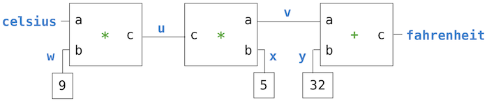
In this figure, we see on the left a multiplier box with three terminals, labeled a, b, and c. These connect the multiplier to the rest of the network as follows: The a terminal is linked to a connector celsius, which will hold the Celsius temperature. The b terminal is linked to a connector w, which is also linked to a constant box that holds 9. The c terminal, which the multiplier box constrains to be the product of a and b, is linked to the c terminal of another multiplier box, whose b is connected to a constant 5 and whose a is connected to one of the terms in the sum constraint.
Computation by such a network proceeds as follows: When a connector is given a value (by the user or by a constraint box to which it is linked), it awakens all of its associated constraints (except for the constraint that just awakened it) to inform them that it has a value. Each awakened constraint box then polls its connectors to see if there is enough information to determine a value for a connector. If so, the box sets that connector, which then awakens all of its associated constraints, and so on. For instance, in conversion between Celsius and Fahrenheit, w, x, and y are immediately set by the constant boxes to 9, 5, and 32, respectively. The connectors awaken the multipliers and the adder, which determine that there is not enough information to proceed. If the user (or some other part of the network) sets the celsius connector to a value (say 25), the leftmost multiplier will be awakened, and it will set u to 25 * 9 = 225. Then u awakens the second multiplier, which sets v to 45, and v awakens the adder, which sets the fahrenheit connector to 77.
Using the Constraint System. To use the constraint system to carry out the temperature computation outlined above, we first create two named connectors, celsius and fahrenheit, by calling the connector constructor.
>>> celsius = connector('Celsius')
>>> fahrenheit = connector('Fahrenheit')
Then, we link these connectors into a network that mirrors the figure above. The function converter assembles the various connectors and constraints in the network.
>>> def converter(c, f):
        """Connect c to f with constraints to convert from Celsius to Fahrenheit."""
        u, v, w, x, y = [connector() for _ in range(5)]
        multiplier(c, w, u)
        multiplier(v, x, u)
        adder(v, y, f)
        constant(w, 9)
        constant(x, 5)
        constant(y, 32)
>>> converter(celsius, fahrenheit)
We will use a message passing system to coordinate constraints and connectors. Constraints are dictionaries that do not hold local states themselves. Their responses to messages are non-pure functions that change the connectors that they constrain.
Connectors are dictionaries that hold a current value and respond to messages that manipulate that value. Constraints will not change the value of connectors directly, but instead will do so by sending messages, so that the connector can notify other constraints in response to the change. In this way, a connector represents a number, but also encapsulates connector behavior.
One message we can send to a connector is to set its value. Here, we (the 'user') set the value of celsius to 25.
>>> celsius['set_val']('user', 25)
Celsius = 25
Fahrenheit = 77.0
Not only does the value of celsius change to 25, but its value propagates through the network, and so the value of fahrenheit is changed as well. These changes are printed because we named these two connectors when we constructed them.
Now we can try to set fahrenheit to a new value, say 212.
>>> fahrenheit['set_val']('user', 212)
Contradiction detected: 77.0 vs 212
The connector complains that it has sensed a contradiction: Its value is 77.0, and someone is trying to set it to 212. If we really want to reuse the network with new values, we can tell celsius to forget its old value:
>>> celsius['forget']('user')
Celsius is forgotten
Fahrenheit is forgotten
The connector celsius finds that the user, who set its value originally, is now retracting that value, so celsius agrees to lose its value, and it informs the rest of the network of this fact. This information eventually propagates to fahrenheit, which now finds that it has no reason for continuing to believe that its own value is 77. Thus, it also gives up its value.
Now that fahrenheit has no value, we are free to set it to 212:
>>> fahrenheit['set_val']('user', 212)
Fahrenheit = 212
Celsius = 100.0
This new value, when propagated through the network, forces celsius to have a value of 100. We have used the very same network to compute celsius given fahrenheit and to compute fahrenheit given celsius. This non-directionality of computation is the distinguishing feature of constraint-based systems.
Implementing the Constraint System. As we have seen, connectors are dictionaries that map message names to function and data values. We will implement connectors that respond to the following messages:
- connector['set_val'](source, value) indicates that the source is requesting the connector to set its current value to value.
- connector['has_val']() returns whether the connector already has a value.
- connector['val'] is the current value of the connector.
- connector['forget'](source) tells the connector that the source is requesting it to forget its value.
- connector['connect'](source) tells the connector to participate in a new constraint, the source.
Constraints are also dictionaries, which receive information from connectors by means of two messages:
- constraint['new_val']() indicates that some connector that is connected to the constraint has a new value.
- constraint['forget']() indicates that some connector that is connected to the constraint has forgotten its value.
When constraints receive these messages, they propagate them appropriately to other connectors.
The adder function constructs an adder constraint over three connectors, where the first two must add to the third: a + b = c. To support multidirectional constraint propagation, the adder must also specify that it subtracts a from c to get b and likewise subtracts b from c to get a.
>>> from operator import add, sub
>>> def adder(a, b, c):
        """The constraint that a + b = c."""
        return make_ternary_constraint(a, b, c, add, sub, sub)
We would like to implement a generic ternary (three-way) constraint, which uses the three connectors and three functions from adder to create a constraint that accepts new_val and forget messages. The response to messages are local functions, which are placed in a dictionary called constraint.
>>> def make_ternary_constraint(a, b, c, ab, ca, cb):
        """The constraint that ab(a,b)=c and ca(c,a)=b and cb(c,b) = a."""
        def new_value():
            av, bv, cv = [connector['has_val']() for connector in (a, b, c)]
            if av and bv:
                c['set_val'](constraint, ab(a['val'], b['val']))
            elif av and cv:
                b['set_val'](constraint, ca(c['val'], a['val']))
            elif bv and cv:
                a['set_val'](constraint, cb(c['val'], b['val']))
        def forget_value():
            for connector in (a, b, c):
                connector['forget'](constraint)
        constraint = {'new_val': new_value, 'forget': forget_value}
        for connector in (a, b, c):
            connector['connect'](constraint)
        return constraint
The dictionary called constraint is a dispatch dictionary, but also the constraint object itself. It responds to the two messages that constraints receive, but is also passed as the source argument in calls to its connectors.
The constraint's local function new_value is called whenever the constraint is informed that one of its connectors has a value. This function first checks to see if both a and b have values. If so, it tells c to set its value to the return value of function ab, which is add in the case of an adder. The constraint passes itself (constraint) as the source argument of the connector, which is the adder object. If a and b do not both have values, then the constraint checks a and c, and so on.
If the constraint is informed that one of its connectors has forgotten its value, it requests that all of its connectors now forget their values. (Only those values that were set by this constraint are actually lost.)
A multiplier is very similar to an adder.
>>> from operator import mul, truediv
>>> def multiplier(a, b, c):
        """The constraint that a * b = c."""
        return make_ternary_constraint(a, b, c, mul, truediv, truediv)
A constant is a constraint as well, but one that is never sent any messages, because it involves only a single connector that it sets on construction.
>>> def constant(connector, value):
        """The constraint that connector = value."""
        constraint = {}
        connector['set_val'](constraint, value)
        return constraint
These three constraints are sufficient to implement our temperature conversion network.
Representing connectors. A connector is represented as a dictionary that contains a value, but also has response functions with local state. The connector must track the informant that gave it its current value, and a list of constraints in which it participates.
The constructor connector has local functions for setting and forgetting values, which are the responses to messages from constraints.
>>> def connector(name=None):
        """A connector between constraints."""
        informant = None
        constraints = []
        def set_value(source, value):
            nonlocal informant
            val = connector['val']
            if val is None:
                informant, connector['val'] = source, value
                if name is not None:
                    print(name, '=', value)
                inform_all_except(source, 'new_val', constraints)
            else:
                if val != value:
                    print('Contradiction detected:', val, 'vs', value)
        def forget_value(source):
            nonlocal informant
            if informant == source:
                informant, connector['val'] = None, None
                if name is not None:
                    print(name, 'is forgotten')
                inform_all_except(source, 'forget', constraints)
        connector = {'val': None,
                     'set_val': set_value,
                     'forget': forget_value,
                     'has_val': lambda: connector['val'] is not None,
                     'connect': lambda source: constraints.append(source)}
        return connector
A connector is again a dispatch dictionary for the five messages used by constraints to communicate with connectors. Four responses are functions, and the final response is the value itself.
The local function set_value is called when there is a request to set the connector's value. If the connector does not currently have a value, it will set its value and remember as informant the source constraint that requested the value to be set. Then the connector will notify all of its participating constraints except the constraint that requested the value to be set. This is accomplished using the following iterative function.
>>> def inform_all_except(source, message, constraints):
        """Inform all constraints of the message, except source."""
        for c in constraints:
            if c != source:
                c[message]()
If a connector is asked to forget its value, it calls the local function forget-value, which first checks to make sure that the request is coming from the same constraint that set the value originally. If so, the connector informs its associated constraints about the loss of the value.
The response to the message has_val indicates whether the connector has a value. The response to the message connect adds the source constraint to the list of constraints.
The constraint program we have designed introduces many ideas that will appear again in object-oriented programming. Constraints and connectors are both abstractions that are manipulated through messages. When the value of a connector is changed, it is changed via a message that not only changes the value, but validates it (checking the source) and propagates its effects (informing other constraints). In fact, we will use a similar architecture of dictionaries with string-valued keys and functional values to implement an object-oriented system later in this chapter.
Continue: 2.5 Object-Oriented Programming