1.7.1   The Anatomy of Recursive Functions

A common pattern can be found in the body of many recursive functions. The body begins with a base case, a conditional statement that defines the behavior of the function for the inputs that are simplest to process. In the case of sum_digits, the base case is any single-digit argument, and we simply return that argument. Some recursive functions will have multiple base cases.

The base cases are then followed by one or more recursive calls. Recursive calls always have a certain character: they simplify the original problem. Recursive functions express computation by simplifying problems incrementally. For example, summing the digits of 7 is simpler than summing the digits of 73, which in turn is simpler than summing the digits of 738. For each subsequent call, there is less work left to be done.

Recursive functions often solve problems in a different way than the iterative approaches that we have used previously. Consider a function fact to compute n factorial, where for example fact(4) computes $4! = 4 \cdot 3 \cdot 2 \cdot 1 = 24$.

A natural implementation using a while statement accumulates the total by multiplying together each positive integer up to n.

>>> def fact_iter(n):
        total, k = 1, 1
        while k <= n:
            total, k = total * k, k + 1
        return total

>>> fact_iter(4)
24

On the other hand, a recursive implementation of factorial can express fact(n) in terms of fact(n-1), a simpler problem. The base case of the recursion is the simplest form of the problem: fact(1) is 1.

These two factorial functions differ conceptually. The iterative function constructs the result from the base case of 1 to the final total by successively multiplying in each term. The recursive function, on the other hand, constructs the result directly from the final term, n, and the result of the simpler problem, fact(n-1).

As the recursion "unwinds" through successive applications of the fact function to simpler and simpler problem instances, the result is eventually built starting from the base case. The recursion ends by passing the argument 1 to fact; the result of each call depends on the next until the base case is reached.

The correctness of this recursive function is easy to verify from the standard definition of the mathematical function for factorial:

While we can unwind the recursion using our model of computation, it is often clearer to think about recursive calls as functional abstractions. That is, we should not care about how fact(n-1) is implemented in the body of fact; we should simply trust that it computes the factorial of n-1. Treating a recursive call as a functional abstraction has been called a recursive leap of faith. We define a function in terms of itself, but simply trust that the simpler cases will work correctly when verifying the correctness of the function. In this example, we trust that fact(n-1) will correctly compute (n-1)!; we must only check that n! is computed correctly if this assumption holds. In this way, verifying the correctness of a recursive function is a form of proof by induction.

The functions fact_iter and fact also differ because the former must introduce two additional names, total and k, that are not required in the recursive implementation. In general, iterative functions must maintain some local state that changes throughout the course of computation. At any point in the iteration, that state characterizes the result of completed work and the amount of work remaining. For example, when k is 3 and total is 2, there are still two terms remaining to be processed, 3 and 4. On the other hand, fact is characterized by its single argument n. The state of the computation is entirely contained within the structure of the environment, which has return values that take the role of total, and binds n to different values in different frames rather than explicitly tracking k.

Recursive functions leverage the rules of evaluating call expressions to bind names to values, often avoiding the nuisance of correctly assigning local names during iteration. For this reason, recursive functions can be easier to define correctly. However, learning to recognize the computational processes evolved by recursive functions certainly requires practice.

1.7.2   Mutual Recursion

When a recursive procedure is divided among two functions that call each other, the functions are said to be mutually recursive. As an example, consider the following definition of even and odd for non-negative integers:

• a number is even if it is one more than an odd number
• a number is odd if it is one more than an even number
• 0 is even

Using this definition, we can implement mutually recursive functions to determine whether a number is even or odd:

Mutually recursive functions can be turned into a single recursive function by breaking the abstraction boundary between the two functions. In this example, the body of is_odd can be incorporated into that of is_even, making sure to replace n with n-1 in the body of is_odd to reflect the argument passed into it:

>>> def is_even(n):
        if n == 0:
            return True
        else:
            if (n-1) == 0:
                return False
            else:
                return is_even((n-1)-1)

As such, mutual recursion is no more mysterious or powerful than simple recursion, and it provides a mechanism for maintaining abstraction within a complicated recursive program.

1.7.3   Printing in Recursive Functions

The computational process evolved by a recursive function can often be visualized using calls to print. As an example, we will implement a function cascade that prints all prefixes of a number from largest to smallest to largest.

>>> def cascade(n):
        """Print a cascade of prefixes of n."""
        if n < 10:
            print(n)
        else:
            print(n)
            cascade(n//10)
            print(n)

>>> cascade(2013)
2013
201
20
2
20
201
2013

In this recursive function, the base case is a single-digit number, which is printed. Otherwise, a recursive call is placed between two calls to print.

It is not a rigid requirement that base cases be expressed before recursive calls. In fact, this function can be expressed more compactly by observing that print(n) is repeated in both clauses of the conditional statement, and therefore can precede it.

>>> def cascade(n):
        """Print a cascade of prefixes of n."""
        print(n)
        if n >= 10:
            cascade(n//10)
            print(n)

As another example of mutual recursion, consider a two-player game in which there are n initial pebbles on a table. The players take turns, removing either one or two pebbles from the table, and the player who removes the final pebble wins. Suppose that Alice and Bob play this game, each using a simple strategy:

• Alice always removes a single pebble
• Bob removes two pebbles if an even number of pebbles is on the table, and one otherwise

Given n initial pebbles and Alice starting, who wins the game?

A natural decomposition of this problem is to encapsulate each strategy in its own function. This allows us to modify one strategy without affecting the other, maintaining the abstraction barrier between the two. In order to incorporate the turn-by-turn nature of the game, these two functions call each other at the end of each turn.

>>> def play_alice(n):
        if n == 0:
            print("Bob wins!")
        else:
            play_bob(n-1)

>>> def play_bob(n):
        if n == 0:
            print("Alice wins!")
        elif is_even(n):
            play_alice(n-2)
        else:
            play_alice(n-1)

>>> play_alice(20)
Bob wins!

In play_bob, we see that multiple recursive calls may appear in the body of a function. However, in this example, each call to play_bob calls play_alice at most once. In the next section, we consider what happens when a single function call makes multiple direct recursive calls.

1.7.4   Tree Recursion

Another common pattern of computation is called tree recursion. As an example, consider computing the sequence of Fibonacci numbers, in which each number is the sum of the preceding two.

This recursive definition is tremendously appealing relative to our previous attempts: it exactly mirrors the familiar definition of Fibonacci numbers. Consider the pattern of computation that results from evaluating fib(6), shown below. To compute fib(6), we compute fib(5) and fib(4). To compute fib(5), we compute fib(4) and fib(3). In general, the evolved process looks like a tree (the diagram below is not a full environment diagram, but instead a simplified depiction of the process). Each blue dot indicates a completed computation of a Fibonacci number in the traversal of this tree.

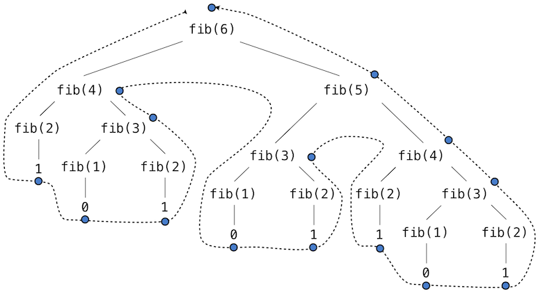
Functions that call themselves multiple times in this way are said to be tree recursive. This function is instructive as a prototypical tree recursion, but it is a terribly inefficient way to compute Fibonacci numbers because it does so much redundant computation. Notice that the entire computation of fib(4) -- almost half the work -- is duplicated. In fact, it is not hard to show that the number of times the function will compute fib(1) or fib(2) (the number of leaves in the tree, in general) is precisely fib(n+1). To get an idea of how bad this is, one can show that the value of fib(n) grows exponentially with n. fib(40) is 63,245,986! The function above uses a number of steps that grows exponentially with the input.

We have already seen an iterative implementation of Fibonacci numbers, repeated here for convenience.

>>> def fib_iter(n):
        """Return the nth Fibonacci number, for n >= 2."""
        predecessor, current = 0, 1   # Fibonacci numbers 1 and 2
        k = 2  # Which Fib number is bound to current?
        while k < n:
            predecessor, current = current, predecessor + current
            k = k + 1
        return current

The state that we must maintain in this case consists of the current and previous Fibonacci numbers, along with the index of the current number. This definition does not reflect the standard mathematical definition of Fibonacci numbers as clearly as the recursive approach. However, the amount of computation required in the iterative implementation is only linear in n, rather than exponential. Even for small values of n, this difference can be enormous.

One should not conclude from this difference that tree-recursive processes are useless. When we consider processes that operate on hierarchically structured data rather than numbers, we will find that tree recursion is a natural and powerful tool. Furthermore, tree-recursive processes can often be made more efficient, as we will see in Chapter 3.

1.7.5   Example: Partitions

The number of partitions of a positive integer n, using parts up to size m, is the number of ways in which n can be expressed as the sum of positive integer parts up to m in increasing order. For example, the number of partitions of 6 using parts up to 4 is 9.

1. 6 = 2 + 4
2. 6 = 1 + 1 + 4
3. 6 = 3 + 3
4. 6 = 1 + 2 + 3
5. 6 = 1 + 1 + 1 + 3
6. 6 = 2 + 2 + 2
7. 6 = 1 + 1 + 2 + 2
8. 6 = 1 + 1 + 1 + 1 + 2
9. 6 = 1 + 1 + 1 + 1 + 1 + 1

We will define a function count_partitions(n, m) that returns the number of different partitions of n using parts up to m. This function has a simple solution as a tree-recursive function, based on the following observation:

The number of ways to partition n using integers up to m equals

1. the number of ways to partition n-m using integers up to m, and
2. the number of ways to partition n using integers up to m-1.

To see why this is true, observe that all the ways of partitioning n can be divided into two groups: those that include at least one m and those that do not. Moreover, each partition in the first group is a partition of n-m, followed by m added at the end. In the example above, the first two partitions contain 4, and the rest do not.

Therefore, we can recursively reduce the problem of partitioning n using integers up to m into two simpler problems: (1) partition a smaller number n-m, and (2) partition with smaller components up to m-1.

To complete the implementation, we need to specify the following base cases:

1. There is one way to partition 0: include no parts.
2. There are 0 ways to partition a negative n.
3. There are 0 ways to partition any n greater than 0 using parts of size 0 or less.

>>> def count_partitions(n, m):
        """Count the ways to partition n using parts up to m."""
        if n == 0:
            return 1
        elif n < 0:
            return 0
        elif m  == 0:
            return 0
        else:
            return count_partitions(n-m, m) + count_partitions(n, m-1)

>>> count_partitions(6, 4)
9
>>> count_partitions(5, 5)
7
>>> count_partitions(10, 10)
42
>>> count_partitions(15, 15)
176
>>> count_partitions(20, 20)
627

We can think of a tree-recursive function as exploring different possibilities. In this case, we explore the possibility that we use a part of size m and the possibility that we do not. The first and second recursive calls correspond to these possibilities.

Implementing this function without recursion would be substantially more involved.